Prerequisites#

A Restricted Boltzmann Machine (RBM) is an energy-based probabilistic graphical model composed of a visible layer and a hidden layer, with no intra-layer connections but full inter-layer connections. Its core idea is to learn the latent feature distribution of data through unsupervised learning.

1. Neural Network Basics#

1.1 Neuron Model#

The artificial neuron is the basic computing unit of a neural network. Given an input vector $\mathbf{x} \in \mathbb{R}^n$ , its output is:

$a = \phi\left( \mathbf{w}^\top \mathbf{x} + b \right)$

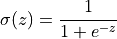
where $\mathbf{w} \in \mathbb{R}^n$ is the weight vector, $b \in \mathbb{R}$ is the bias term, and $\phi(\cdot)$ is the activation function. In probabilistic generative models the Sigmoid activation is commonly used:

$\sigma(z) = \frac{1}{1 + e^{-z}}$

1.2 Energy-Based Models#

Unlike feed-forward networks, Energy-Based Models (EBMs) define a probability distribution over data through a scalar energy function $E(\mathbf{x}; \theta)$ :

$P(\mathbf{x}; \theta) = \frac{\exp(-E(\mathbf{x}; \theta))}{Z(\theta)}$

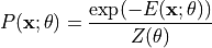
where the partition function is:

$Z(\theta) = \sum_{\mathbf{x}} \exp(-E(\mathbf{x}; \theta))$

It ensures proper normalization. States with lower energy correspond to higher probability.

2. Boltzmann Machine Structure#

Visible layer (v): the explicit representation of input data (e.g. pixel values).
Hidden layer (h): extracted latent features.
Weight matrix (w): weights connecting visible and hidden layers.
Biases: visible-layer bias (b) and hidden-layer bias (c).

A Boltzmann Machine (BM) is fully connected, whereas the Restricted Boltzmann Machine removes intra-layer connections, making Gibbs sampling far more efficient.

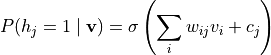
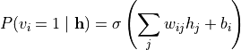
Thanks to the restricted structure, hidden variables are mutually independent given the visible variables, with conditional probability:

$P(h_j = 1 \mid \mathbf{v}) = \sigma\left( \sum_i w_{ij} v_i + c_j \right)$

Similarly,

$P(v_i = 1 \mid \mathbf{h}) = \sigma\left( \sum_j w_{ij} h_j + b_i \right)$

3. Energy Function and Probability Distribution#

3.1 Energy Function#

The RBM energy function is defined as:

$E(\mathbf{v}, \mathbf{h}) = -\mathbf{v}^T \mathbf{W} \mathbf{h} - \mathbf{b}^T \mathbf{v} - \mathbf{c}^T \mathbf{h}$

where $\mathbf{v}, \mathbf{h}$ are the states of the visible and hidden layers, $\mathbf{W}$ is the connection weight matrix, and $\mathbf{b}, \mathbf{c}$ are the first-order coefficients.

The joint probability distribution is given by the Boltzmann distribution:

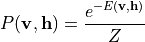
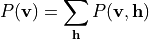
$P(\mathbf{v}, \mathbf{h}) = \frac{e^{-E(\mathbf{v}, \mathbf{h})}}{Z}$

where $Z$ is the partition function (normalization factor). The marginal distribution over the visible layer is:

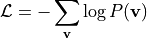
$P(\mathbf{v}) = \sum_{\mathbf{h}} P(\mathbf{v}, \mathbf{h})$

Parameters $W,b,c$ are learned by maximizing the likelihood. The objective is the negative log-likelihood:

$\mathcal{L} = -\sum_{\mathbf{v}} \log P(\mathbf{v})$

Contrastive Divergence (CD) is used to approximate the gradient; the update rule is:

$\Delta W_{ij} = \epsilon \left( \langle v_i h_j \rangle_{\text{data}} - \langle v_i h_j \rangle_{\text{recon}} \right)$

where $\epsilon$ is the learning rate, and $\langle \cdot \rangle_{\text{data}}$ , $\langle \cdot \rangle_{\text{recon}}$ denote expectations under the data and reconstruction distributions, respectively.

3.2 Gradient Derivation#

The probability of an energy model can be written as:

$p(x; \theta) = \frac{1}{Z} \tilde{p}(x; \theta)$

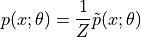
Its gradient is:

$\nabla_\theta \log p(x; \theta) = \nabla_\theta \log \tilde{p}(x; \theta) - \nabla_\theta \log Z$

The gradient of the partition function is hard to compute directly:

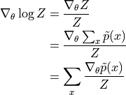
$\nabla_\theta \log Z &= \frac{\nabla_\theta Z}{Z} \\ &= \frac{\nabla_\theta \sum_x \tilde{p}(x)}{Z} \\ &= \sum_x \frac{\nabla_\theta \tilde{p}(x)}{Z}$

For models that guarantee $p(x) > 0$ for every $x$ , we can replace $\tilde{p}(x)$ with $\exp(\log \tilde{p}(x))$ .

$\frac{\sum_x \nabla_\theta \exp(\log \tilde{p}(x))}{Z} &= \frac{\sum_x \exp(\log \tilde{p}(x)) \nabla_\theta \log \tilde{p}(x)}{Z} \\ &= \frac{\sum_x \tilde{p}(x) \nabla_\theta \log \tilde{p}(x)}{Z} \\ &= \sum_x p(x) \nabla_\theta \log \tilde{p}(x) \\ &= \mathbb{E}_{x \sim p(x)} \nabla_\theta \log \tilde{p}(x)$

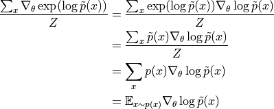
Putting it together,

$\nabla_\theta \log p(x; \theta) = \nabla_\theta \log \hat{p}(x; \theta) - \mathbb{E}_{x \sim p(x; \theta)} \nabla_\theta \log \hat{p}(x; \theta)$

In the second term $p(x; \theta)$ is the distribution predicted by the model, while the first term in training is under the real data distribution. Thus the equation can be rewritten as:

$\nabla_\theta \log p(x; \theta) = \mathbb{E}_{x \sim p_{\text{data}}} \nabla_\theta \log \hat{p}(x; \theta) - \mathbb{E}_{x \sim p_{\text{model}}} \nabla_\theta \log \hat{p}(x; \theta)$

Considering the Boltzmann-machine energy function, we can easily obtain:

$\nabla_W \log \hat{p}(x; W) = v h^\mathrm{T}$

One only needs to obtain the values of $v$ and $h$ under $p_{\text{data}}$ and $p_{\text{model}}$ respectively to compute the gradient, namely:

$\Delta W_{ij} = \epsilon \left( \langle v_i h_j \rangle_{\text{data}} - \langle v_i h_j \rangle_{\text{recon}} \right)$